Constrained optimization provides the mathematical language and solver technology to search the space of legal decisions and pick the one (or several) that best meet your goals.
Why Constrained Optimization Matters
Finding a valid solution within a set of structured tradeoffs is exactly what modern solvers handle well.
Budgets, staffing caps, legal rules, equipment counts, minimum coverage levels, preferred work patterns, and fatigue thresholds all create boundaries that any feasible plan must respect.
In workforce scheduling, especially when staff express shift preferences, you must strike a balance: honor as many preferences as possible while never violating licensing, rest, and coverage requirements.
Core Building Blocks
Before choosing a solver, it helps to define the pieces that all constrained optimization models share.
Decision variables
Unknowns you control. Example: x=1 if a nurse works a given shift.
Objective function
What you optimize. Minimize cost, maximize preference satisfaction, reduce overtime, or combine them.
Constraints
Mathematical statements that must hold. Hard constraints define legality. Soft constraints encode preferences and can be modeled with penalties or additional variables.
Feasible region
All assignments that satisfy the hard constraints. The solver searches within this region.
Optimal solution
A feasible assignment that yields the best objective value found (global or local, depending on solver type).
Solver Landscape: What Is Available and When To Use It
Below is a narrative overview of common solver families and what they are good for.
Linear Programming (LP)
Handles continuous decision variables with linear objective and linear constraints. Extremely fast at large scale. Ideal for resource allocation, blending, capacity planning, and network flow problems where fractional solutions are acceptable or later rounded. Some structured LPs (network simplex, min cost flow) produce integer solutions naturally because of total unimodularity.
Typical solvers: Gurobi, CPLEX, FICO Xpress, Google OR-Tools Linear Solver (GLOP), COIN-OR Clp.
Mixed Integer Linear Programming (MILP or MIP)
Extends LP by allowing binary or integer variables. This is the workhorse for most scheduling, assignment, facility location, production sequencing, and routing formulations. If your decision is yes/no, on/off, or whole-number counts, you likely need MILP.
Typical solvers: Gurobi, CPLEX, Xpress, CBC (open source), SCIP (open source), OR-Tools MIP wrapper.
Constraint Programming (CP)
Designed for highly combinatorial problems with complex logical and temporal constraints that may be awkward to express linearly. CP engines propagate constraints to prune the search tree early. Good for detailed rostering, shift patterns, sequencing with calendars, and problems with many discrete relationships but relatively weak cost-optimization structure.
Typical solvers: OR-Tools CP-SAT (hybrid CP + SAT + MILP), IBM CP Optimizer, Choco, OptaPlanner (rule/score-based CP hybrid).
CP-SAT Hybrid (Boolean + Integer)
Google OR-Tools CP-SAT deserves its own mention. It blends SAT solving, CP propagation, and integer programming. Outstanding for large binary scheduling and rostering problems with complex Boolean logic, calendar patterns, and priority objectives.
Quadratic and Conic Optimization (QP, MIQP, SOCP)
When your objective includes squared terms (variance, risk, distance) or cone constraints (robust optimization, certain energy dispatch problems), QP or SOCP solvers come into play. Mixed integer variants exist but are harder to solve.
Typical solvers: Gurobi (QP, MIQP), CPLEX, Mosek (conic), OSQP (QP), ECOS (conic).
Nonlinear Programming (NLP, MINLP)
Necessary when relationships are curved (nonlinear cost curves, pharmacokinetic dose response, nonlinear staffing productivity). Smooth NLPs are tractable; nonsmooth or mixed integer nonlinear problems are difficult and often handled with decomposition or heuristics.
Typical solvers: IPOPT, SNOPT, Knitro, Bonmin (MINLP), Couenne.
Metaheuristics and Hybrid Approaches
Genetic algorithms, simulated annealing, tabu search, large neighborhood search, and greedy randomized methods are useful when models are huge, highly nonlinear, or you only need good (not provably optimal) solutions quickly. Often combined with MIP or CP to polish results.
Libraries: OR-Tools large neighborhood search (vehicle routing heritage), OptaPlanner score director, custom Python heuristic frameworks.
When a Linear Solver Is Ideal
Even if your organization works with complex rosters, there are many planning layers where a pure linear formulation is fast, transparent, and effective. Here are practical use cases.
- Allocating aggregate nursing hours by specialty across days of the week when fractional hours are acceptable for planning and later rounded in detail scheduling.
- Determining weekly operating room block time by service line based on forecast case hours and target utilization.
- Budget allocation across departments to maximize expected patient coverage subject to spending caps.
- Pharmacy compounding and supply mixing where ingredient proportions must meet nutritional or dosage bounds.
- Network distribution of medical supplies across multiple hospitals minimizing transport cost with demand and capacity constraints.
- Staff training hour allocation: how many total continuing education hours per role this quarter to satisfy requirements at minimum backfill cost.
- Pre-balancing floating staff pools across regions before running detailed shift-level assignment.
- Energy consumption scheduling in hospital facilities where loads can be modeled continuously (pre-chiller capacity, HVAC modulation) under demand charge constraints.
- Ambulance positioning using continuous probability coverage models that are later discretized into posts.
- High-level scenario planning: if elective volume grows 15 percent, what continuous increase in staff hours keeps coverage above threshold?
If any of these decisions can be expressed as linear relationships and do not depend on a large number of yes/no assignment choices, an LP will solve fast and scale gracefully.
A Robust Example: Nurse Shift Preference Scheduling
Imagine that every week a hospital needs to publish a new schedule for the week. The nurses submit preferred shifts. Lets look at how this can be solved with constrained optimization.
Problem Context
You must schedule N nurses across a 7 day horizon with 3 shifts per day (morning, day, night). Each nurse has:
- One or more required skills (ICU, OR, MedSurg, Pediatrics).
- Availability (cannot work on certain days).
- Requested shifts ranked 1, 2, 3.
- Limits on max weekly hours and consecutive nights.
- Minimum rest between shifts (for example 10 hours).
The nurses indicate their preferred shifts for each day of the week:
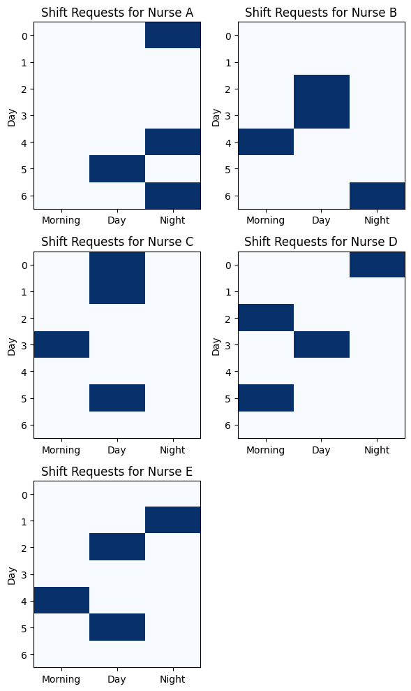
It is important to remember that the solver must also meet coverage targets by unit and shift. Some units require at least one charge nurse per shift.
Sets & Data
- Nurse roster – the full list of individual nurses.
- Planning calendar – the days in the scheduling horizon.
- Shift types – for example, day, evening, and night.
- Hospital units – such as ICU, pediatrics, or surgery.
- Qualification map – which nurses hold the credentials to work in each unit.
- Availability map – which shifts each nurse can actually work.
- Preference levels – how strongly each nurse would like a particular shift.
- Staffing targets – the minimum number of nurses and charge nurses required for every unit and shift.
- Charge‑nurse flag – which nurses are certified to act as charge nurses.
Decision Variables
- Assignment flag – indicates whether a specific nurse is scheduled in a particular unit on a given day and shift.
- Daily‑work flag – tracks whether a nurse works at all on a given day.
- Preference shortfall indicator – records when a nurse’s stated preference is not met (optional).
- Rest‑violation indicator – highlights when mandatory rest periods are broken (penalized heavily).
Core Constraints
- Qualified and available – a nurse can be assigned only if they are certified for the unit and free to work that shift.
- One unit per shift – a nurse cannot be placed in more than one unit during the same shift.
- Weekly hour limit – total scheduled hours for any nurse must stay within contract limits.
- Mandatory rest – if two shifts are too close together, the nurse cannot be assigned to both.
- Unit coverage – every unit must meet its minimum nurse count on every shift.
- Charge‑nurse coverage – each unit must also meet its minimum requirement for charge nurses.
- Daily tracking – flags ensure the system knows whether a nurse is on duty each day.
- Consecutive‑day limit – no nurse may exceed the allowed number of working days in a row.
Objective
The schedule aims to respect three competing goals:
- Honor preferences – give nurses the shifts they most want whenever possible.
- Protect fairness – distribute unpopular or weekend shifts evenly and avoid excessive overtime.
- Minimize penalty costs – heavily discourage violations of rest rules or other critical policies.
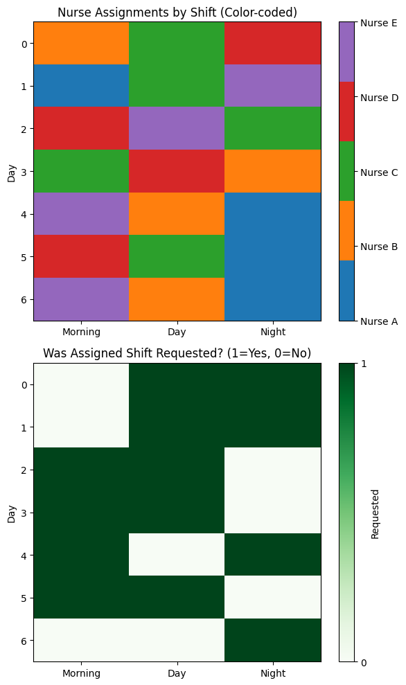
A practical approach is to satisfy coverage first, then maximize preference fulfillment, and finally smooth out fairness. Modern solvers such as Gurobi can handle these layered priorities within a single multi‑objective run or through successive passes that refine the schedule step by step.
Handling Soft Requirements at Scale
As the problem grows (hundreds of staff, multiple roles, rotating patterns) you will need strategies to manage soft rules without exploding solve time.
Penalty variables
Introduce nonnegative slack with costs for violating soft requests. Easy to scale.
Layered solve
Solve first for feasibility, then fix coverage and reoptimize to improve preferences.
Large neighborhood search
Start with a feasible roster, then repeatedly “destroy and repair” segments to improve satisfaction scores.
Reinforcement learning weight tuning
Use RL to learn which soft weights produce the best long term staff satisfaction and low override counts. (See our companion resource article on RL plus forecasting.)
Human in the loop
Expose a ranked list of near-optimal swap suggestions so schedulers can apply judgment without breaking feasibility.
Modeling Tips That Save You Pain
- Clean your availability data. Inconsistent shift lengths or missing credentials create infeasible models.
- Aggregate where you can. Pre-assign fixed rules (such as union-mandated holidays) before the solver runs.
- Keep objective weights scaled similarly. Very large big-M numbers can degrade solver performance.
- Use warm starts. Feed last week’s schedule to jump-start the search.
- Profile constraint groups. Remove or relax rules that rarely bind.
What Success Looks Like
A good constrained optimization deployment reduces manual scheduling hours, improves staff satisfaction, and gives leadership knobs to explore tradeoffs.
In the nurse preference example, hospitals see fewer overruns, better weekend balance, and faster response when availability changes. Stakeholders trust the results and can audit why decisions were made because the model encodes policy transparently.
At Front Analytics we design and implement optimization pipelines that fit your data environment and operational goals. Whether you need a lightweight LP for capacity planning or a full mixed integer and constraint hybrid to schedule thousands of staff with preferences, we can help you model, tune, deploy, and govern the solution. Learn how we can help solve your scheduling or resource allocation challenge.